累积矩阵 Accumulating Matrices
讨论层级矩阵累积、非均匀缩放导致的 skew,以及矩阵分解修正方案。
累积矩阵 Accumulating Matrices
从概念上来说,累积变换并最终得到 世界变换 最简单的方式就是链式的一路递归相乘它们各自父节点的变换矩阵,经典的图形程序大多都是这样操作的
Matrix ToMatrix(Transform transform) {
    // First, extract the rotation basis of the transform
    // 也可以直接使用 四元数公式展开法 直接得到旋转矩阵
    Vector x = Vector(1, 0, 0) * transform.rotation; // Vec3 * Quat (right vector)
    Vector y = Vector(0, 1, 0) * transform.rotation; // Vec3 * Quat (up vector)
    Vector z = Vector(0, 0, 1) * transform.rotation; // Vec3 * Quat (forward vector)

    // Next, scale the basis vectors
    // 如果上一步使用了 公式展开 此处应该构造缩放矩阵
    x = x * transform.scale.x; // Vector * float
    y = y * transform.scale.y; // Vector * float
    z = z * transform.scale.z; // Vector * float

    // Extract the position of the transform
    Vector t = transform.position;

    // Create matrix
    return Matrix(
        x.x, x.y, x.z, 0, // X basis (& Scale)
        y.x, y.y, y.z, 0, // Y basis (& scale)
        z.x, z.y, z.z, 0, // Z basis (& scale)
        t.x, t.y, t.z, 1  // Position
    );
}

Matrix GetWorldMatrix(Transform t) {
    Matrix local = ToMatrix(t);       // 由 pos/rot/scale 组装
    if(t.parent)                      // 递归到根
        return local * GetWorldMatrix(t.parent);
    return local;
}
注意,这里使用了 行向量-左乘体系 row vector / left multiply
约定 向量写法 组合规则(局部 → 世界) 列向量 / 右乘 v' = M · v世界矩阵 = Parent · Local 先算父节点,再右乘子节点 行向量 / 左乘 v' = v · M世界矩阵 = Local · Parent 先算子节点,再左乘父节点 常见列向量的变换组合顺序是
T · R · S;行向量是S · R · T但是本质上都是先 缩放,再 旋转,最后 位移
从表面上看,该代码按预期运行,但一旦引入 非均匀缩放,马上就会产生问题,例如如果我们有如下层级关系的变换
Transform A- position: (0, 0, 0)
- rotation: (0, 0, 0)
- scale: (2, 1, 1) 非均匀缩放
Transform B- position: (2, 2, 0)
- rotation: (0, 0, 38)
- scale: (1, 1, 1)
Transform C- position: (0, 0, 0)
- rotation: (0, 0, 0)
- scale: (1, 1, 1)
当我们旋转 B,本该绕 Z 轴转,却变成 倾斜 / 剪切(Skew)
父节点的非均匀缩放会把子节点的局部正交基带入非正交世界基
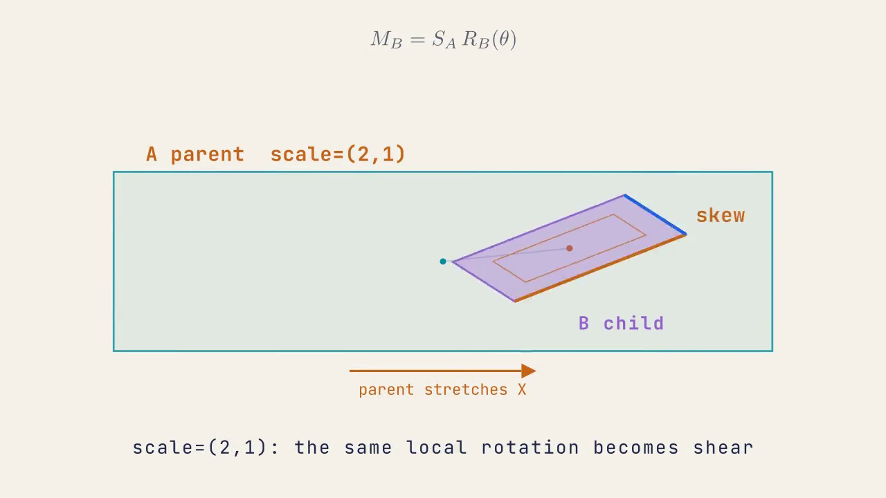
这是因为 A 的 非均匀缩放 (2,1,1) 将它的 局部矩阵 的 个 基向量 拉伸成不等长,它的子对象 B 在计算自己的 世界变换 时,拿到的就是这样的 非正交矩阵,这将导致 “旋转 + 剪切” 参杂在一起,而如果 B 还有更多的后代,那么任何后代节点都会继承这个 非正交基向量,动作越多畸变越严重
解决 Skew
不存在 “便宜” 的 one-liner 修复法,两个常见的手段是
- 纯 TRS 链路
不直接存储 矩阵,每帧用 position / quaternion / scale 重新拼矩阵,这并不是简单的分开存储它们(我们已经这么做了),而是在整条递归链路上分开累积它们,并最终在送往 GPU 时才将它们合并为矩阵(因为 GPU 需要矩阵) - 矩阵分解
将父变换的 矩阵进行 矩阵分解,重新组合
| 传统方案(矩阵链乘) | 纯 TRS 方案 | |
|---|---|---|
| 层级累积 | 每级都把 T·R·S 先拼成 M_local, 然后 M_world = parent M_world × M_local | 每级分别把 pos / quat / scale 递推到世界:worldPos = pPos + pRot*(pScale ⊙ pos)worldQuat = pQuat × quatworldScale = pScale ⊙ scale |
| 链路中保存 | 始终是 4 × 4 矩阵(T+R+S+Shear 都混在一起) | 始终是 三个独立分量流,链路里从不出现 4×4 |
| GPU 前一步 | 直接把父级递推得到的 M_world 写进 UBO / SSBO / constant buffer | 到达渲染阶段才一次性M_world = T(worldPos)·R(worldQuat)·S(worldScale) |
| 副作用 | 父级若含非均匀缩放,再被子级旋转→易产生 Skew / Shear | 几乎不产生剪切;数值稳定;读取/写入局部 TRS 便宜 |
也就是说,矩阵链式相乘 是
而 TRS 链 是
-
整条层级链只递推 世界平移 、世界旋转 、世界缩放
这里的 是按分量相乘(Hadamard)。
-
最后一刻才把这三样重新排成
可以发现,它是 分量递推 的形式,与 矩阵链式相乘 再分解是等价的
| 步骤 | 纯 TRS 递推 | 乘-分解 |
|---|---|---|
| 局部→世界平移 | 乘完再取分解的 T 项,结果相同(分解把平移直接读出) | |
| 局部→世界旋转 | 剪切被投影掉,分解后的 R 即为正交矩阵 | |
| 局部→世界缩放 | 分解提取的对角块就是各向缩放,同样为分量相乘 |
它们都丢弃了 剪切变换
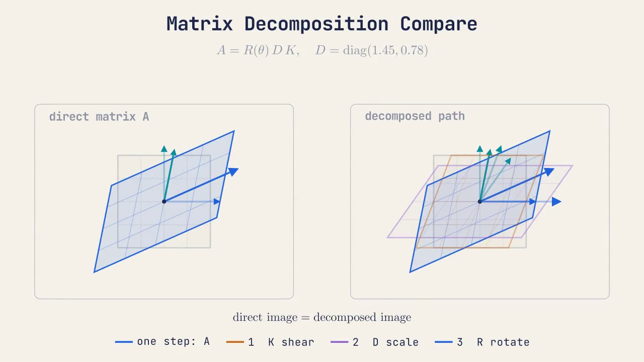
矩阵分解 Matrix Decomposition
直接把父子矩阵 链式相乘 的这种方法虽然很省事,但一旦父节点有 非均匀缩放,子节点做旋转就将导致 剪切伪影,子元素的旋转变换会导致其 倾斜 (skew) 而不是旋转
解决这个 非均匀缩放 问题的唯一方法是通过 矩阵分解,其思路是,将最终存在 倾斜 skew 问题 的矩阵分解为 位置、旋转、缩放 和 倾斜 分量,分解完所有这些分量后,忽略 倾斜,创建一个仅包含 位置、旋转 和 缩放 的新矩阵
这种类型的分解在 Shoemake 和 Duff 的论文 Matrix Animation and Polar Decomposition 以及 Shoemake 在 Graphics Gems IV 的章节 Polar Matrix Decomposition 中均有描述
显然矩阵分解是一项昂贵的操作,对性能有重大影响
这种方法拥有 开源代码,它的接口看起来像这样
typedef struct {
    HVect t;  /* Translation components */
    Quat  q;  /* Essential rotation   */
    Quat  u;  /* Stretch rotation   */
    HVect k;  /* Stretch factors    */
    float f;  /* Sign of determinant    */
} AffineParts;

void decomp_affine(HMatrix A, AffineParts *parts);
我们可以通过调用 decomp_affine 函数从变换矩阵中得到不含 剪切 shearing 的 位移 t,旋转 q,缩放 k,这些值可以用于构建一个新的变换矩阵
Matrix GetWorldMatrix(Transform transform) {
    Matrix localMatrix = ToMatrix(transform);
    Matrix worldMatrix = localMatrix;

    if (transform.parent != NULL) {
        Matrix parentMatrix = GetWorldMatrix(transform.parent);
        worldMatrix = localMatrix * parentMatrix;

        if (ContainsNonUniformScale(transform.parent)) {
            AffineParts decomp = decomp_affine(worldMatrix, &decomp);

            Transform temp;
            temp.parent = NULL;
            temp.position = decomp.t;
            temp.scale = decomp.k;
            temp.rotation = decomp.q;

            worldMatrix = ToMatrix(temp);
        }
    }

    return worldMatrix;
}
使用上述代码,我们可以修复 倾斜伪影,使旋转按预期工作
decomp_affine 函数的内容是这样的,我们来看看它如何将 的 齐次变换矩阵 分解为独立的几部分
void decomp_affine(HMatrix A, AffineParts *parts) {
    HMatrix Q, S, U;
    Quat p;
    float det;
    parts->t = Qt_(A[X][W], A[Y][W], A[Z][W], 0);
    det = polar_decomp(A, Q, S);
    if (det<0.f) {
        mat_copy(Q,=,-Q,3);
        parts->f = -1;
    }
    else {
        parts->f = 1;
    }
    parts->q = Qt_FromMatrix(Q);
    parts->k = spect_decomp(S, U);
    parts->u = Qt_FromMatrix(U);
    p = snuggle(parts->u, &parts->k);
    parts->u = Qt_Mul(parts->u, p);
}| 代码行 | 作用 | 结果写进 AffineParts 的字段 |
|---|---|---|
parts->t = Qt_(A[X][W] … ) | 直接把矩阵最后一列(平移分量)拷出来 | t(平移向量) |
det = polar_decomp(A, Q, S) | 对原矩阵做极分解: • Q 得到正交矩阵(含旋转+可能的翻转)• S 得到对称矩阵(含缩放+剪切)同时返回行列式 det | - |
若 det<0 | 行列式 < 0 说明 Q 带镜像翻转,需要把它整反(乘以 –1)并记 f = –1;否则 f = 1 | f(是否带翻转) |
parts->q = Qt_FromMatrix(Q) | 把整理好的正交矩阵 Q 转成四元数 | q(纯旋转) |
parts->k = spect_decomp(S, U) | 对 S 做特征分解,剥离剪切:• 得到本征值 → 各轴缩放向量 k• 得到本征向量矩阵 U → “附加旋转” | k(缩放) |
parts->u = Qt_FromMatrix(U) | 把 U 转为四元数 | u(附加旋转) |
p = snuggle(u,&k); u = Qt_Mul(u,p) | k、u 这对值有 24 种等价写法,snuggle 调整它们,使后续插值连续稳定;u 最后再右乘一次校正用的四元数 p | u、修正后的 k |
极分解 把任意可逆矩阵拆成「正交 * 对称」两部分,是去掉剪切的常用办法
- 对称矩阵: 继续执行 特征分解 将 缩放(特征值) 与剩余剪切分开,并把 缩放 值挤进向量
k - 正交矩阵:通过检测其 行列式 的 正负性 来判定是否需要把旋转 反转,如果需要反转,则把符号记录到
f
最终还需要经过 snuggle 调整,因为 k、u 不是唯一的,需要选一组“连贯”的值,避免动画插值时突然跳轴或符号颠倒,snuggle 直接修改 k 并返回一个需要与 u 相乘的 四元数,不过在我们的用例里,我们并不关心 u,也不会对它进行插值,所以当 k 被矫正以后,我们就得到了所有想要的
最终我们得到
t—— 纯平移q—— 纯旋转(四元数,已经排除了镜像)k—— XYZ 三轴缩放系数u—— 与缩放相关的补偿旋转(通常在做插值时一起参与计算)f—— ±1,记录有没有镜像翻转
这个过程在动画、骨骼绑定、形变空间插值(Dual Quaternion / DQS 等)里都很有用
分解过程的数学分析
假设我们想进行上述 仿射变换 affinate transformation 分解并将它存储至矩阵 ,我们可以将 分解为一个 线性变换 linear transformation 和一个 位移 translation 的形式
分解位移
分解位移是最容易的,首先设 ,然后将 除了最后一列之外全部置零,然后设 ,但是这次我们只将最后一列代表 位移 的部分置零(和之前正好相反),如此一来,我们得到分解
列主序(column-major)+ 列向量后乘(post-multiplication),OpenGL/GLM 最常用的约定, 齐次变换矩阵 的 平移分量 必须放在最右侧那一列
典型环境 向量写法 乘法顺序 位移在几列(行) 列向量 / 后乘 OpenGL、GLM、Shader GLSL 最后一列 (Songho) 行向量 / 先乘 DirectX(旧)、某些游戏引擎 最后一行 (Stack Overflow) 二者在数学结果上等价;只是把“基向量”和“位移向量”存成列还是行,及乘法顺序互为转置而已
我们得到只含 位移 的 平移矩阵 ,以及不含 平移 矩阵的
极分解 Polar Decomposition
接着,我们对上一步得到 做 极分解
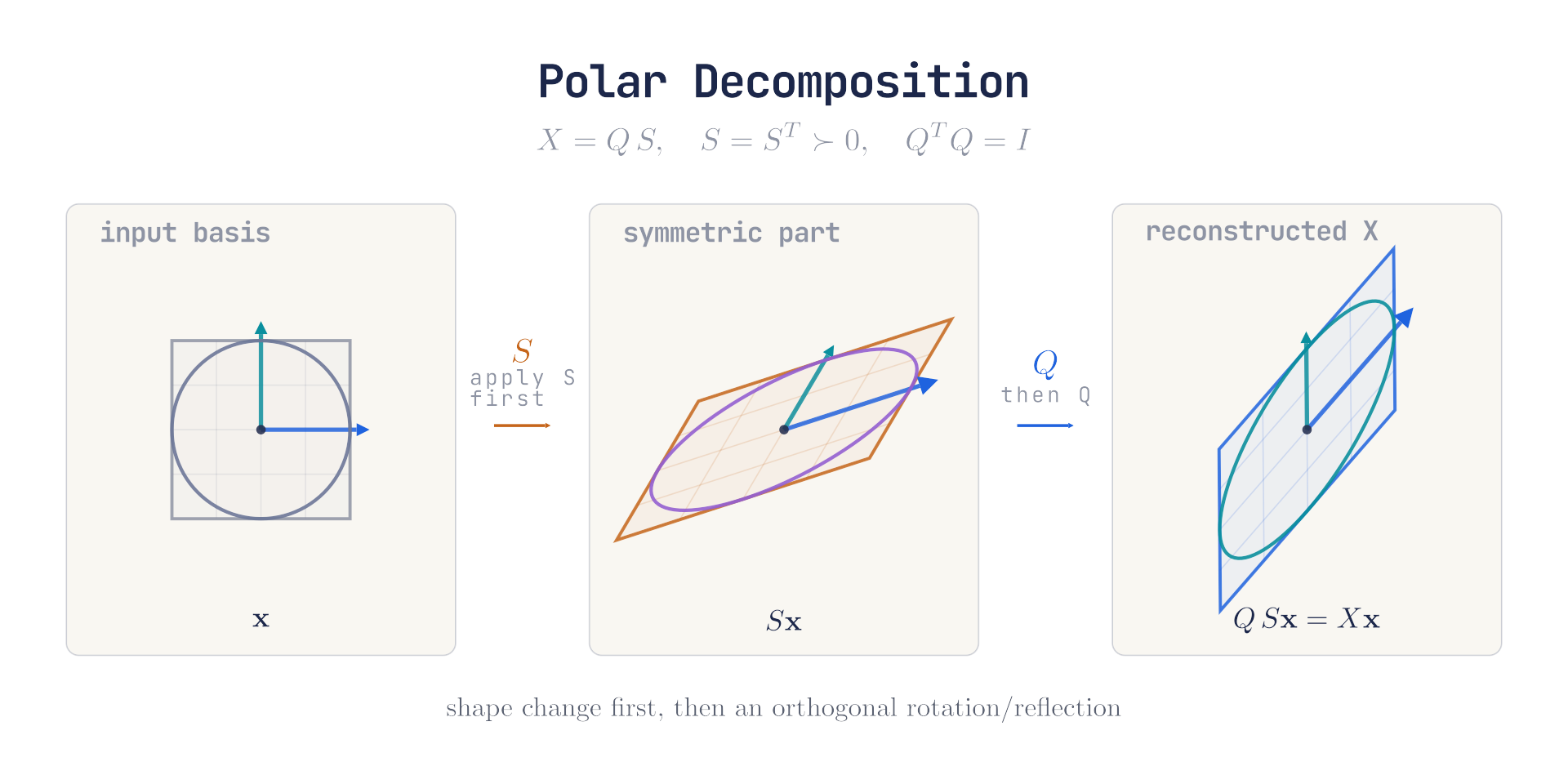
- 是 正交矩阵,描述了 旋转 或者 旋转+镜像翻转
- 是 对称正定矩阵,描述了 缩放和剪切,也就是 形变
将 极分解 结果代入上一步,得到
从 中识别镜像翻转
我们可以根据 行列式 来判断 旋转矩阵 中是否含有 镜像翻转
所以我们可以对 执行分解
- ,所以 表示 不翻转/翻转
- 是 纯旋转
再次回代,得到
谱分解 (特征分解) Spectral / Eigen Decomposition
对称矩阵 包含了 缩放 和 剪切,我们对它进行 特征分解
- 是 对角矩阵,表示 各轴缩放
- 是 正交矩阵 (因为 是一个 对称矩阵,所以它的 特征向量 矩阵是 正交矩阵),表示包含 剪切 的 附加旋转
我们一般使用 QR 算法 进行 特征分解
这里的分解结果 和 并非唯一的,对于同一个 ,它的特征分解结果一共有 种等价组合 (轴重排 × 轴符号 × 旋转 );若要执行 跨帧插值,则需要为每帧挑选一组彼此 “最接近” 的 ,也就是枚举 种合法的组合,计算将 变换到 的旋转 ,选择 旋转角最小 的组合,这就是代码 snuggle() 的工作
我们再次进行回代
最终
我们最终得到完整的分解
我们只需要使用 三个部分来构建我们 去除剪切 的变换矩阵,将其他不需要的完全忽略
- 通常将翻转矩阵 放进缩放矩阵 中
分解位移
一个代表 3D 仿射变换的 矩阵可以被分解为一个 3D 线性变换 和一个 位移 的形式
struct FactorTranslationResult {
    Matrix T; // Translation
    Matrix X; // Linear transformation
};

FactorTranslationResult FactorTranslation(Matrix M) {
    FactorTranslationResult result;

    result.T = Matrix4();
    result.T[12] = M[12];
    result.T[13] = M[13];
    result.T[14] = M[14];

    result.X = M;
    result.X[12] = 0;
    result.X[13] = 0;
    result.X[14] = 0;

    return result;
}
取决于矩阵在内存里的“主序”(row-major vs column-major)
4 × 4 矩阵的一维下标 column-major(OpenGL/GLM 默认) row-major(C 数组 / 大多数 DX 示例) 0‥3 第 0 列 (r0c0‥r3c0) 第 0 行 (r0c0‥r0c3) 4‥7 第 1 列 第 1 行 8‥11 第 2 列 第 2 行 12‥14 第 3 列的前三个元素 → Tx, Ty, Tz 第 3 行的前三个元素 → Tx, Ty, Tz 15 r3c3 (= 1) r3c3 (= 1)
- 列主序(column-major)下标 12-14 落在 最后一列,对应逻辑坐标 。这是 OpenGL-style 的“位移列”。
- 行主序(row-major)下标 12-14 则落在 最后一行,对应 。这是 DirectX-style 的“位移行”。
因为这两个布局把同一批浮点排在同样的 12-14 槽位,只看下标无法区分主序;必须结合库/API 文档或乘法写法来判断:
vec4 v1 = M * v0;   // 常见于列向量-后乘体系(OpenGL)
vec4 v1 = v0 * M;   // 常见于行向量-先乘体系(传统 DirectX)
所以,若你的矩阵库采用列主序(GLM、Eigen 默认设置等),
T[12]~T[14]是“最后一列”;若采用行主序,它们才是“最后一行”。
极分解
由于 和 矩阵的求逆成本很低 (40 – 60 flop) ,所以我们一般使用 迭代算法 来做它们的 极分解
- 是 正交矩阵
- 是 对称正定 矩阵
首先我们初始化
然后反复 取平均
将矩阵与自己的 逆转置 求平均,能逐步消除不正交的成分,迭代若干次 (一般上界是 步) 或者当 足够小就收敛
struct PolarDecompResult {
    Matrix Q; // 旋转/翻转矩阵
    Matrix S; // 对称矩阵(缩放+剪切)
};

bool PolarDecompositionEarlyOut(Matrix Q, Matrix Qprev) {
    return (Q - Qprev); // 全部分量足够接近 0
}

PolarDecompResult PolarDecomposition(Matrix X) {
    Matrix Q = X;                       // Q0
    for (int i = 0; i < 20; ++i) {      // 最多 20 次
        Matrix Qprev = Q;
        Matrix Qit   = Inverse(Transpose(Q)); // Q_i^{-T}
        Q = 0.5f * (Q + Qit);                // 取平均
        if (PolarDecompositionEarlyOut(Q, Qprev))
            break;                           // 收敛就退出
    }
    result.Q = Q;
    // result.S = Inverse(Q) * X;
    // 可以用正交矩阵的转置来替代其逆 计算更快
    result.S = Transpose(Q) * X;
    // 或者,使用 “正交性” 容差,在未成功收敛到正交时时兜底
    // if (fabs(det(Q) - 1.0f) < 1e-3f &&
    //     norm(Q.transpose()*Q - I) < 1e-3f)
    //     S = Q.transpose() * X;
    // else
    //     S = inverse(Q) * X;   // 退化或未收敛时兜底

    return result;
}
Inverse(Transpose(Q)) 就是 ,有了它我们可以很容易的计算
因为最终 是 正交矩阵,所以
我们还需要从 中去除 镜像 部分,从而得到 纯旋转,这需要检查
struct FactorRotationResult {
    Matrix F; // ±I,det<0 时为 -I
    Matrix R; // 纯旋转矩阵
};

FactorRotationResult FactorRotation(Matrix Q) {
    float f = 1.0f;
    if (Det(Q) < 0) {   // 含镜像
        f = -1.0f;
        Q = Q * -1;     // 元素逐分量取负,去掉翻转
    }
    result.F = diag(f,f,f,1); // ±I
    result.R = Q;            // 现在 det(R)=+1
    return result;
}
若 则 已经是 纯旋转,否则要把 全取负号,相当于提出一个翻转矩阵 ,余下的 就是 正交旋转
对于 矩阵的 极分解,也有 借助四元数 的方案
QR 分解
QR 分解 将一个矩阵 分解为
- 是 正交矩阵
- 是 上三角矩阵
QR 分解 是 QR 算法(求 特征值/特征向量)以及数值稳定线性求解的基础,求解大型矩阵的 QR 分解 往往采用 Givens 旋转 和 House Holder 反射,但是可能最朴素简单的方法是 Gram-Schmidt 正交化
取 的三列向量 ,令
再分别 Normalize 三个向量,得到的 就是 的列,虽然 Gram-Schmidt 正交化 的效率不高,但是对于小型矩阵,它的开销是可以接受的
而且当矩阵尺寸很小时,Gram-Schmidt 的实现最简单、寄存器占用最少,也易于在 GPU/ SIMD 里展开流水线。唯一需要注意的是数值稳定性:若输入列向量接近线性相关,需要改用 “改进 Gram-Schmidt” 或做一次交叉积+归一化的快速基构造
步骤 浮点操作 (FLOPs) 两次向量投影(点乘+标量乘+减) ≈ 24 FLOP (MIT DSpace) 三次向量归一化(点乘+rsqrt+乘) ≈ 30 FLOP (MIT DSpace, 维基百科) 合计 ≈ 50–60 FLOP 若矩阵几乎奇异,可先做一次快速
cross()重建,也可以看看 Pixar 的这篇 论文
Vector x(A[0], A[1], A[2]);
Vector y(A[4], A[5], A[6]);
Vector z(A[8], A[9], A[10]);

y = y - ProjectionV3(x, y);
z = (z - Projection(x, z)) - Projection(y, z);

x = Normalize(x);
y = Normalize(y);
z = Normalize(z);

// 写回 result.Q 的 0~2、4~6、8~10 元素
由于 的 正交性,求 很简单
也就是
result.R = Transpose(result.Q) * A;完整代码
struct QRDecompResult {
    Matrix Q; // Q is an orthogonal matrix
    Matrix R; // R os an upper triangular matrix
}

QRDecompResult QRDecomposition(Matrix A) {
    QRDecompResult result;

    Vector x(A[0], A[1], A[2]);
    Vector y(A[4], A[5], A[6]);
    Vector z(A[8], A[9], A[10]);

    y = y -  ProjectionV3(x, y); // y minus projection of y onto x
    z = (z - Projection(x, z)) - Projection(y, z);

    x = Normalize(x);
    y = Normalize(y);
    z = Normalize(z);

    result.Q[0] = x[0]; resuly.Q[1] = x[1]; result.Q[2] = x[2];
    result.Q[4] = y[0]; result.Q[5] = y[1]; result.Q[6] = y[2];
    result.Q[8] = z[0]; result.Q[9] = z[1]; result.Q[10]= z[2];

    result.R = Transpose(result.Q) * A;

    return result;
}
谱分解 Spectral Decomposition (特征分解)
我们需要把 极分解 得到的 对称矩阵 用 特征分解 来分解得到
- 是 正交矩阵,列向量都是 的 特征向量
- 是 对角矩阵,对角线元素是对应的 特征值
- 是 的 转置 (等于 逆)
这种分解是 不唯一 的, 和 的行可以被任意重新排列,甚至取反符号,最终得到的结果仍然相同
计算 实对称矩阵 的 特征值/特征向量 也可以使用 迭代方法,具体来说,是使用 QR-分解 进行迭代
首先,初始化
然后对 做 QR 分解
令 ,并把本轮迭代得到的 连乘累积进 ,进行反复迭代,直到 的 下三角 足够接近 (或者到达 迭代上限,一般也是 次),此时迭代收敛,收敛后
- 的 对角线 即为 特征值,将它写入
- 累乘得到的 就是全部 特征向量
struct SpectralDecompositionResult{
    Matrix U;   // 特征向量矩阵
    Matrix K;   // 对角存特征值
    Matrix Ut;  // U 的转置
};

bool SpectralDecompositionEarlyOut(Matrix A){
    int idx[]{4,8,9,12,13,14};   // 下三角的 6 个元素
    for(auto i: idx)
        if(!EpsilonCompare(A[i],0)) return false;
    return true;                 // 都接近 0 说明已趋近对角
}

SpectralDecompositionResult SpectralDecomposition(Matrix S){
    result.U = Identity();
    Matrix A = S;

    for(int i=0;i<20;++i){
        auto decomp = QRDecomposition(A); // 第 1 步
        result.U = result.U * decomp.Q;   // 第 2 步:累积特征向量
        A        = decomp.R * decomp.Q;   // 第 3 步:A ← RQ

        if(SpectralDecompositionEarlyOut(A)) break;
    }

    result.Ut = Transpose(result.U);      // 保存 U^T

    result.K = Identity();
    result.K[0]=A[0]; result.K[1]=A[1]; result.K[2]=A[2]; // 对角=特征值

    return result;
}
此处 QR分解 使用普通的 Gram-Schmidt 正交化,后续 snuggle 步骤会在 种等价组合里挑一组最 “平滑” 的 和
Spectral Adjustment 谱调整
因为 特征分解 得到的 并不唯一,同一个 至少有 种可能的 组合,如果我们想在两帧之间平滑插值矩阵,就必须从这 个组合里挑选一组,使得当前帧的 与上一帧的 尽可能的接近 (旋转角最小)
之所有有 种有效组合可能,是因为对于 的 实对称 矩阵:
-
轴交换:将 特征向量 的分量排列顺序任意交换 → 种
-
成对翻转符号:一次性改变两个分量的符号,也不会改变结果
组合编号 X 轴 Y 轴 Z 轴 行列式 ① +X +Y +Z +1 ② −X −Y +Z (−1)·(−1)·(+1) = +1 ③ −X +Y −Z (−1)·(+1)·(−1) = +1 ④ +X −Y −Z (+1)·(−1)·(−1) = +1 可以发现,行列式结果不变,我们依然位于 右手系
将两种操作的可能数相乘,我们得到 ,这些操作不会改变 的正确性,却会让 旋转到完全不同的方向,于是插值时可能发生 “跳轴” 或 180° 翻面
我们的目标是让相邻帧的 差异最小,给定两帧的形变矩阵 和 (假设 是上一帧的, 是当前帧的)
-
先各自做 特征分解 得到 和
-
枚举 的 个 变体
我们对于每一个 变体 都计算 所需的 角度,也就是从上一帧的 姿态 旋转到这一帧的 候选姿态 所需旋转的 角度,然后选取所需 角度 最小的那个 作为最终的我们知道,如果将 非零向量 用 旋转到 世界坐标,则可以得到 在 下的 姿态
同理,将 用 也旋转到 世界坐标,得到 在 下的 姿态
然后,我们需要找到一个 相对旋转 ,将 姿态 旋转到 姿态
显然 姿态 是上一帧数据已经决定了的,无法改变,但是不同的 候选旋转矩阵 将得到不同的 姿态 ,从而使得进行 的姿态变化所需的 相对旋转 需要旋转的 角度 不同,我们希望这个角度最小,那么首先要计算 相对旋转
然后我们可以将 转换为 四元数 来比较 旋转角,四元数的 分量大则旋转角度小,也就是说找到使得 相对旋转 对应 四元数 分量最大的那个 ,即为我们最后选定最佳
- 越小, 越接近
-
最后,同步 重排/翻转 的主对角元素,以匹配选择的
最终得到的 与 在插值时就不会突然大角度跳变,这就是之前代码中的 snuggle 函数
// ❶ 24 个 3×3 置换-翻符号矩阵预先写在 permutations[24]
Matrix U1 = input.U;        // 上一帧或当前基准
Matrix U2 = input.Ut;       // 本帧原始 U (待调整)

// ❷ 遍历全部 24 组合
for(i=0;i<24;++i){
    Matrix U2p = permutations[i] * U2;        // 应用置换/翻符号
    Quaternion q = ToQuat(  U2p * U1ᵀ );       // 相对四元数
    if(q.w > best) { best=q.w; save=i; }      // cos(θ/2) 最大 = 旋转角最小
}

// ❸ 选中最佳组合
Matrix U2_best = permutations[save] * U2;
Matrix Ut_best = U2_bestᵀ;
Matrix K_best  = diag( K 原值按同样置换/翻符号重排 );

// ❹ 输出
return { U2_best, K_best, Ut_best };
只要对称矩阵连贯变化,遍历 24 种离散候选就足以找到最平滑的一条轨迹,并且对于 尺度,枚举+比较 的代价微乎其微
struct SpectralAdjustmentResult {
    Matrix U; // Each basis vector is an eigenvector
    Matrix K; // Contains eigenvalues on main diagonal
    Matrix Ut; // Transpose of U
}

SpectralAdjustmentResult SpectralDecompositonAdjustment(SpectralDecompositionResult input) {
  Matrix U1 = input.U;
  Matrix U1t = input.Ut;

  Matrix[24][9] m_permutations = [
    // Permutation 0: x, y, z
    [ 1, 0, 0,  0, 1, 0,  0, 0, 1 ],
    [-1,-0,-0, -0,-1,-0,  0, 0, 1 ],
    [ 1, 0, 0, -0,-1,-0, -0,-0,-1 ],
    [-1,-0,-0,  0, 1, 0, -0,-0,-1 ],
    // Permutation 1: x, z, y
    [-1,-0,-0,  0, 0, 1,  0, 1, 0 ],
    [-1,-0,-0, -0,-0,-1, -0,-1,-0 ],
    [ 1, 0, 0,  0, 0, 1, -0,-1,-0 ],
    [ 1, 0, 0, -0,-0,-1,  0, 1, 0 ],
    // Permutation 2: y, x, z
    [-0,-1,-0,  1, 0, 0,  0, 0, 1 ],
    [-0,-1,-0, -1,-0,-0, -0,-0,-1 ],
    [ 0, 1, 0,  1, 0, 0, -0,-0,-1 ],
    [ 0, 1, 0, -1,-0,-0,  0, 0, 1 ],
    // Permutation 3: y, z, x
    [ 0, 1, 0,  0, 0, 1,  1, 0, 0 ],
    [-0,-1,-0, -0,-0,-1,  1, 0, 0 ],
    [ 0, 1, 0, -0,-0,-1, -1,-0,-0 ],
    [-0,-1,-0,  0, 0, 1, -1,-0,-0 ],
     // Permutation 4: z, x, y
    [ 0, 0, 1,  1, 0, 0,  0, 1, 0 ],
    [-0,-0,-1, -1,-0,-0,  0, 1, 0 ],
    [ 0, 0, 1, -1,-0,-0, -0,-1,-0 ],
    [-0,-0,-1,  1, 0, 0, -0,-1,-0 ],
    // Permutation 5: z, y, x
    [-0,-0,-1,  0, 1, 0,  1, 0, 0 ],
    [-0,-0,-1, -0,-1,-0, -1,-0,-0 ],
    [ 0, 0, 1,  0, 1, 0, -1,-0,-0 ],
    [ 0, 0, 1, -0,-1,-0,  1, 0, 0],
  ];

  float x = input.K[0];
  float y = input.K[5];
  float z = input.K[10];

  Vector[6][3] eigen_value_permutations = [
    [ x,  y,  z], // Permutation 0
    [ x,  z,  y], // Permutation 1
    [ y,  x,  z], // Permutation 2
    [ y,  z,  x], // Permutation 3
    [ z,  x,  y], // Permutation 4
    [ z,  y,  x], // Permutation 5
  ];

  int saved_index = -1
  int saved_value = -1

  // The rotation taking U1 into U2 is U1t * U2
  for (int i = 0; i < 24; ++i) {
    Matrix U2 = m_permutations[i];
    Matrix U12 = U1t * U2;

    Quaternion QU12 = ToQuaternion(U12);

    // Optimize for largest w, which is smallest angle of rotation
    if (saved_index == -1 || QU12.w > saved_value) {
      saved_value = QU12.w
      saved_index = i
    }
  }

  Matrix U2t = Transpose(m_permutations[saved_index])
  var index = saved_index/4; // Integer division (floor this)

  SpectralAdjustmentResult result;
  result.U = Mul3(U1, U2t);
  result.K = Matrix(
    eigen_value_permutations[index][0], 0, 0, 0,
    0, eigen_value_permutations[index][1], 0, 0,
    0, 0, eigen_value_permutations[index][2], 0,
    0, 0, 0, 1
  );
  result.Ut = Transpose(result.U)

  return result;
}
这段代码使用了 行向量 和 矩阵右乘,而不是我们推导中使用的 列向量 和 矩阵左乘
仿射分解 Affine Decomposition
我们已经拥有了所有所需的函数,接下来只需要组装最终的 仿射分解
| 阶段函数 | 作用 | 产物 |
|---|---|---|
FactorTranslation | 拆出平移 T,并留下 3 × 3 线性部分 X | T, X |
PolarDecomposition | 把 X 分成正交矩阵 Q(旋转或翻转)和对称矩阵 S(缩放+剪切) | Q, S |
FactorRotation | 再把 Q 拆成 • ±I(翻转标记 F) • 纯旋转 R | F, R |
SpectralDecomposition | 对称矩阵 S → 特征分解 | U, K, Uᵀ |
SpectralDecompositionAdjustment | 在 24 组置换/符号里挑一组,使新 U 与前一帧 U 的旋转角最小(snuggle) | 调整后的 U, K, Uᵀ |
AffineDecomposition 函数看起来像下面这样
AffineDecompositionResult AffineDecomposition(Matrix M) {
    // ① 平移
    auto trans  = FactorTranslation(M);          // 得 T, X
    // ② 极分解
    auto polar  = PolarDecomposition(trans.X);   // 得 Q, S
    // ③ 抽翻转 & 纯旋转
    auto rot    = FactorRotation(polar.Q);       // 得 F, R
    // ④ 特征分解
    auto spec   = SpectralDecomposition(polar.S);// 得 U, K, Ut
    // ⑤ snuggle 调整
    auto snug   = SpectralDecompositionAdjustment(spec);

    AffineDecompositionResult res;
    res.T  = trans.T;        // 平移
    res.F  = rot.F;          // ±1 翻转标记
    res.R  = rot.R;          // 纯旋转矩阵
    res.U  = snug.U;         // stretch-rotation
    res.K  = snug.K;         // 缩放对角
    res.Ut = snug.Ut;        // Uᵀ
    return res;
}
Shoemake 在 Graphics Gems IV 用的是
| 字段 | 意义 |
|---|---|
| T | 平移向量 |
| F | 行列式符号 (±1) |
| q | 纯旋转四元数 (R) |
| u | stretch-rotation 四元数 (U) |
| k | 伸缩向量(K 的三对角) |
ShoemakeResult ConvertToShoemake(AffineDecompositionResult a){
    ShoemakeResult s;
    s.T = Vector3(a.T[12], a.T[13], a.T[14]);
    s.F = a.F[0];                      // ±1
    s.q = ToQuaternion(a.R);           // R → 四元数
    s.u = ToQuaternion(a.U);           // U → 四元数
    s.k = Vector3(a.K[0], a.K[5], a.K[10]);
    return s;
}